
Convolutional neural network 2: architecture
Convolutional neural network provides one of the best classification results for images. In the previous post, you had the opportunity to learn what a convolution is and how to classify a CIFAR-10 dataset using a simple densly connected neural network. By the way, we have obtained accuracy of 47% on the test set.
In the second part of the tutorial we go further:
- we explain the basic concepts and the architecture of convolutional neural networks,
- we build a simple convnet and check how it works on the CIFAR-10 dataset,
- and we briefly explain what an overfitting is – an issue that we will deal with in the third part of this tutorial.
This post is the second part of the tutorial, so if you haven’t read the first one, I encourage you to read it first.
Convolutional neural network – architecture
Let’s start with the fact that a convolutional neural network consists of two sub-nets. The first of them converts the input tensor. The second one is a classic densely connected neural network, terminated with a layer, which classifies the input data into N classes – as in the example from the first part of the tutorial. The convolutional subnet usually processes three-dimensional data, i.e. unprocessed except for normalization. A densely connected network, on the other hand, requires data flattened to one dimension.
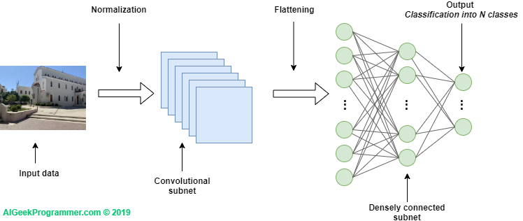
Figure no. 1: Convolutional neural network – high-level architecture
If we adopt this somewhat artificial division into sub-nets (and knowing from other post how to classify image data using a classic neural network), we can basically focus further on the first element only, i.e. on the convolutional part.
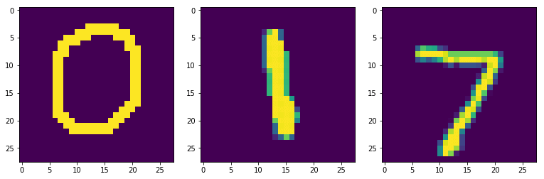
Before we go deeper into the architecture of the convolutional network, let’s think for a moment why Convnets handle images so well? If you read my post about handwriting classification, you may remember that all the numbers were more or less in the center of the picture. It looked something like this:
The neural network did well with the classification, being sure that what is most interesting will always be in the center of the image. But wait, what if the digit were shifted to one side? Like this:
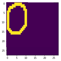
Probably a classic neural network, in addition trained on centrally located digits, would not be able to handle such data. There is a term “translational invariance”. This means that we can recognize an object as the right object, even if its appearance or location has changed to some extent: by shifting, rotating, changing the size, colors, brightness, etc. As in the example above, when we moved zero to the upper left corner, and yet for the human brain it is unquestionably still zero. For a non-translational-invariance neural network, it will be a non-zero object – probably impossible to classify for a network trained on centered symbols. It is noteworthy that the word “translational” is a bit confusing. This is not about translation at all, but rather about transitioning. It was taken from geometry, where it means shifting each pixel in the same way.
Convnets are insensitive to location because their central element is the convolution operation, which involves processing each part of the image with the same filter value. In other words: the convolution does not look at the center of the image or any other area. It runs with the filter throughout entire image, and reports characteristic values in places where it finds an interesting feature.
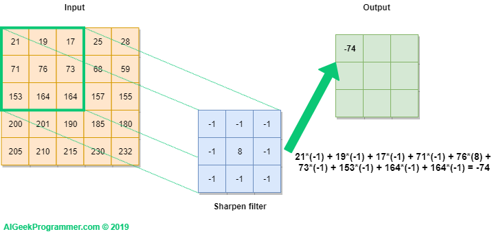
Figure no. 2: convolution – step no. one
Figure no. 2 presents graphically how we perform the convolution operation on a 5×5 pixel image labeled Input, using a 3×3 size filter. The filter was initialized with values that have already appeared in the first part of the tutorial, when we tried to sharpen the edges of an image. The filter is projected onto the image (green frame), and then the value of each pixel of the image is multiplied by the corresponding filter value. As a result, we get the value of -74. Calculations were presented under the output.
In the next step, the filter is moved one position to the right and the calculations are repeated. As a result we get the value of -96.

Figure no. 3: convolution – step no. two
For the last step we get the value of -43, as shown in Figure 4 below.
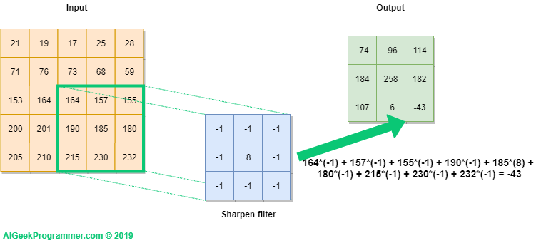
Figure no. 4: convolution – step no. nine
The filter runs all over the input, from left to right and from top to bottom, ultimately filling the output with values.
Figure no. 5: moving the filter through the image
As you can see, as a result of image convolution we can get values below 0, as well as greater than 255. However, we should remember that the purpose of convolution in the neural network is to detect the image features, not visualization after processing with the filter. Hence, it doesn’t really matter until we want to display the image after the convolution (and this happens quite rarely during the training process). If we want to visualize some intermediate state, we should first shift the values, and only in the second step truncate those above 255 to 255, and those below 0 to the value of 0. The issue of: with what value should we shift data is quite complicated and goes beyond the scope of this tutorial. If you are interested in that, please refer to this thread on stackoverflow first.
In summary, data after convolution become insensitive to the location of the object. No matter where it is in fact located, a convolution will be able to find it and return a characteristic set of data for it. The set which is recognizable later by the densly connected neural network. In this sense, Convnets are insensitive to changes in the location of the object and this is one of the main reasons why they classificate images so well.
Like a classic neural sub-net, a convolutional sub-net can be multi-layered. This means that each subsequent layer is able to find more image features. What’s more, each layer of convolution is also multidimensional, because for each layer N filters are defined (see Figure 6 below). Filter values are differently initialized for each of them and they can therefore find better or worse image features important for correct classification. The back propagation algorithm will reduce the importance of inefficient filters, and promote those that support proper classification. Therefore, after many, many iterations, we will have a set of effective filters. Effective in terms of helping the network correctly classify images, and ultimately correctly generalize the classification process.

Figure no. 6: multilayered convolutional network
Another important element of Convnets is the implementation of the so-called maxpooling operation. What is maxpooling is also best to explain visually.

Figure no. 7: maxpooling operation
We analyze the values of four adjacent pixels, select the largest value and it becomes the output / result of the operation. In the next step, we move the operation window to the next group of pixels and repeat the calculations. Unlike convolution, maxpooling windows do not overlap. Therefore, in our example, the next window will be pixels: 114, 105, 182 and 75.
Maxpooling can also be done on a larger sample, e.g. 3×3, 4×4, etc. Note that M x M maxpooling reduces the size of the image by M2. So the 32 x 32 image (1024 pixels), after 2×2 maxpooling will have the dimension of 16×16 = 256 pixels, or 22 times less.
What is a purpose of maxpooling? You’ve already learned the main reason above. Dimensionality is reduced without loss of information relevant to the classification, which simplifies the problem computationally. After performing the convolution (here in the sense: after applying the filter to a given area of the image), we are only interested in whether a significant feature was found in a given area or not. We are not interested in every single pixel value after convolution, but only those values that give a strong answer (strong hint) for our network. Therefore, we look at the values of neighboring pixels and choose the largest – the most important value from them. Furthermore, maxpooling helps identify the elements of the image that are most visible. As a result, we also achieve a higher level of “translational invariance”.
In addition to the maxpooling operation, there is also an average pooling (we calculate the average instead of the maximum) and minpooling, but they are not widely used in Convnets.
Dimensioning of convolutional neural network
As you may have noticed in Figures 2 to 5, the convolution on a 5×5 image with a 3×3 filter resulted in a new 3×3 “image”. Hence the simple conclusion that the convolution may change the dimensions of processed data and it is worth understanding how these dimensions change and how to control these changes. Since I am trying to use the Keras API on the blog, I will use the code line, which we will see later, and which defines the parameters of one of the convolutional layers:
Convolution2D(filters=32, kernel_size=(3,3), activation='relu',padding='same')
The above code creates a convolutional layer with 32 filters, each with 3×3 dimension, and the output from the layer additionally goes through the relu activation function. The padding option is important for this problem, set here to the same value, which means that after the image will be converted, it will have the same size. How is this possible? As the name suggests, we use an artificially added margin (padding), filled with zeros. Keras and Tensorflow offer two ways to handle margins: same and valid.
The valid mode was seen in the examples shown in Figures 2 to 5. The filter does not go outside the image area and thus, the output image is smaller. There is even a simple formula for this. If the image is D x D (in our example 5 x 5) and the filter is N x N (here: 3 x 3), then the size of the resulting image can be calculated from the formula: D – N + 1. For our example it will be 5 – 3 + 1 = 3.
The “same” mode preserves the size of the image after processing by convolution. So that input and output from the convolutional layer will be of the same size. To achieve this, Keras and other frameworks choose the margin size so that the filter passes the image with the margin as many times as the size of the input image. In our case, Keras will add one pixel of margin (padding) to the 5 x 5 image.

Figure 8 – padding types
It is worth noting that for small images – such as in the CIFAR-10 dataset – padding in same mode could be better, so that the size of the output image from the convolution does not drop too quickly, because then we will not be able to add the second and subsequent convolutional layers or perform maxpooling.
Example of dimensioning
Based on what we learned above, let’s try to trace the dimensions in a simple convolutional network. Let’s assume that it will consist of 3 convolution operations, two maxpooling operations and two classic densely connected layers. Also:
- Conv1: padding = “valid”, filter size: 5×5, number of filters: 16
- Maxpool1: 2×2
- Conv2: padding = “same”, filter size: 3×3, number of filters: 8
- Maxpool2: 2×2
- Conv3: padding = “valid”, filter size: 3×3, number of filters: 4
- Dense1: number of neurons at the output: 50
- Dense2: number of neurons at the output: 10 (we classify into 10 classes)
Assuming that we have an image from the CIFAR-10 dataset at the input, how will the sizes change?
- Conv1: the image has a size of 32x32x3 and we perform convolution on it with a 5×5 filter in the valid mode. Here it should be noted that a 5×5 filter is applied to each color channel and eventually added up. The resulting tensor size will therefore be 32-5 + 1 = 28×28. There are 16 filters. Hence, the output from Conv1 will be a 28x28x16 tensor.
- Maxpool1 will reduce the size of each dimension twice. Hence, the output from this layer will be a 14x14x16 tensor.
- Conv2: in this layer we are convolving in the same mode, so it will not change the dimensions of the image. There are 8 filters. Hence the output from Conv2 will be a 14x14x8 tensor.
- Maxpool2 will reduce the size of each dimension twice. Hence, the output from this layer will be a 7x7x8 tensor.
- Conv3: we do a convolution in valid mode, with a 3×3 filter. The resulting tensor size will therefore be 7-3 + 1 = 5×5. There are 4 filters. Hence the output from Conv3 will be a 5x5x4 tensor.
- Dense1: we need to flatten the data to move them to the densely connected neural network. The result is a vector of size 5 * 5 * 4 = 100. It will be the entrance to the first layer of the neural network. It has 50 neurons at the output and this will be the size of the input vector to the last layer – Dense 2.
- Dense2: on the input it receives data of size 50, on the output it has 10 neurons that classify the result with the softmax function.
Classification of the CIFAR-10 dataset
I believe so much theory is enough 😉 and we are ready to try to build a simple convolutional neural network and use it to classify the CIFAR-10 dataset. We will see if we can beat the previous result (47%) obtained with the densely connected neural network.
This time I will use Google Colaboratory environment as we have easy access to the GPU processor there.
Because I want to use tensorflow 2.x, and on the day of writing this post (December 2019) the default version in Colab is still 1.x, besides standard imports we need to add an indication of the expected version of the Tensorflow library.
import numpy as np
%tensorflow_version 2.x
import tensorflow
import matplotlib.pyplot as plt
%matplotlib inline
>>> TensorFlow 2.x selected.
We import the Keras library, cifar-10 dataset and normalize data in the range of -0.5 to 0.5:
from tensorflow import keras
print(tensorflow.__version__)
print(keras.__version__)
>>> 2.1.0-rc1
>>> 2.2.4-tf
from tensorflow.keras.datasets import cifar10
(x_train,y_train), (x_test,y_test) = cifar10.load_data()
x_train.shape
>>> (50000, 32, 32, 3)
print(x_train.min(), "-", x_train.max())
>>> 0 - 255
x_train = (x_train / 255.0) - 0.5
x_test = (x_test / 255.0) - 0.5
print(x_train.min(), "-", x_train.max())
>>> -0.5 - 0.5
Next, we import the classes that we will need to build and train the model:
from tensorflow.keras.models import Sequential
from tensorflow.keras.optimizers import SGD
from tensorflow.keras.layers import Convolution2D, MaxPool2D, Flatten, Dense
from tensorflow.keras.utils import to_categorical
Time to build a model from imported classes. Model building using the Keras API is simple and you can experiment with various architectures. You will quickly notice however, that a diagnosis of whether the changes are in favor or not, is not so simple, as even such a simple convolutional neural network requires considerable computing power and more importantly – your time to wait for a result.
As for the proposed architecture, it will consist of:
- two convolutional layers, each with 64 filters,
- followed by 2×2 MaxPool layer,
- then another two convolutional layers, each with 32 filters,
- and the second layer of 2×2 maxpooling,
- and finally the last pair of convolutions, with 16 filters each.
- Since the images in the cifar-10 dataset are small, all convolutional layers operate with a 3×3 filter and use padding in the same mode, so as not to reduce the size of processed data too quickly.
- As each convolutional layer (like the classic densely connected layer) is a linear one, we add an activation function to the output of each of them, which introduces an additional non-linearity – so liked by neural networks.
- The densely connected subnet expects flattened data, hence the Flatten layer.
- The model ends with three Dense layers, of which the first two have the relu function as an activation, and the third one classifies the result into one of 10 classes using the softmax function.
model = Sequential([
Convolution2D(filters=64, kernel_size=(3,3), input_shape=(32,32,3), activation='relu', padding='same'),
Convolution2D(filters=64, kernel_size=(3,3), activation='relu', padding='same'),
MaxPool2D((2,2)),
Convolution2D(filters=32, kernel_size=(3,3), activation='relu', padding='same'),
Convolution2D(filters=32, kernel_size=(3,3), activation='relu', padding='same'),
MaxPool2D((2,2)),
Convolution2D(filters=16, kernel_size=(3,3), activation='relu', padding='same'),
Convolution2D(filters=16, kernel_size=(3,3), activation='relu', padding='same'),
Flatten(),
Dense(units=512, activation="relu"),
Dense(units=64, activation="relu"),
Dense(units=10, activation="softmax")
])
Keras offers two useful ways to visualize the model. The first is the summary method, which will not only show the output data shapes on each layer, but will also calculate the complexity of the model by calculating the number of network parameters.
model.summary()
Model: "sequential"
_________________________________________________________________
Layer (type) Output Shape Param #
=================================================================
conv2d (Conv2D) (None, 32, 32, 64) 1792
_________________________________________________________________
conv2d_1 (Conv2D) (None, 32, 32, 64) 36928
_________________________________________________________________
max_pooling2d (MaxPooling2D) (None, 16, 16, 64) 0
_________________________________________________________________
conv2d_2 (Conv2D) (None, 16, 16, 32) 18464
_________________________________________________________________
conv2d_3 (Conv2D) (None, 16, 16, 32) 9248
_________________________________________________________________
max_pooling2d_1 (MaxPooling2 (None, 8, 8, 32) 0
_________________________________________________________________
conv2d_4 (Conv2D) (None, 8, 8, 16) 4624
_________________________________________________________________
conv2d_5 (Conv2D) (None, 8, 8, 16) 2320
_________________________________________________________________
flatten (Flatten) (None, 1024) 0
_________________________________________________________________
dense (Dense) (None, 512) 524800
_________________________________________________________________
dense_1 (Dense) (None, 64) 32832
_________________________________________________________________
dense_2 (Dense) (None, 10) 650
=================================================================
Total params: 631,658
Trainable params: 631,658
Non-trainable params: 0
_________________________________________________________________
The second way presents the model in graphic form, with the option of presenting the shapes of input and output data.
from tensorflow.keras.utils import plot_model
plot_model(model, 'model_info.png', show_shapes=True)
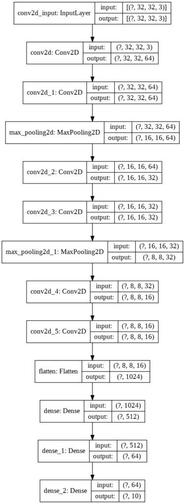
Figure 9 – graphic representation of the model
Next, we need to determine the optimizer, the loss function and the metrics that we want to collect during the training process. Both: the type of optimizer and its parameters (here learning rate and momentum) – are so called hyperparameters of the model. They will affect its behavior, speed and effectiveness of learning. These are obviously one of the many hyperparameters of our model. The architecture and complexity of the model itself is already critical to the network effectiveness. The size of the filters, their number, type of padding, activation functions, data normalization method, maxpooling conversions – these are other hyperparameters. The number of combinations is really large. It is worth taking advantage of the tips that can be easily found on the internet and start with hyperparameters that have already been checked and provided good effects, and then try to improve the results experimentally.
optim = SGD(lr=0.001, momentum=0.5)
model.compile(optimizer=optim, loss='categorical_crossentropy', metrics=['accuracy'])
After compiling the model, we can start the training process. With the parameters given below, it will last from several minutes to several dozen minutes (depends on the processing unit available). Note that results of the fit method are returned to the history object, which will collect data, so that afterwards we can display training process characteristics. I have also added the validation_split parameter to the fit method, which specifies how much of the training data is reserved for the validation process. This process takes place after each epoch, showing what effects the training process on the training dataset gives on the validation set (which the network has not seen during learning in this epoch).
history = model.fit(
x_train,
to_categorical(y_train),
epochs=80,
validation_split=0.15,
verbose=1
)
The final verification takes place on the test set that the network has not previously seen:
eval = model.evaluate(x_test, to_categorical(y_test))
eval
>>> [1.6473742815971375, 0.6954]
As you can see, by using the convolutional neural network, we were able to increase the accuracy of classification from 47% to nearly 70%.
However, some interesting things can be observed using the data collected in the history object:
plt.plot(history.history['accuracy'])
plt.plot(history.history['val_accuracy'])
plt.title('Model accuracy')
plt.ylabel('Accuracy')
plt.xlabel('Epoch')
plt.legend(['Train', 'Validation'], loc='upper left')
plt.show()
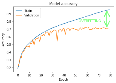
Figure 10 – learning and overfitting process
Figure 10 shows the training results on the training set (blue line) and results on the validation set (orange line). As you can see around the 15th epoch both datasets began to obtain different results. The accuracy for the training set gradually increased, eventually reaching around 95%. Meanwhile, validation has done a lot worse. The same applies to the test set.
What does it mean? Well, we are dealing here with so called overfitting (marked by a green arrow in Figure 10): the model almost perfectly learned how to recognize objects from the training set, but could not generalize this knowledge in such a way as to correctly classify objects previously unseen. This is not a good situation, because the network will not cope well with data outside of the training process. Fortunately, there are several techniques that reduce overfitting – we’ll cover them in the third part of the tutorial.
Thanks for reading! If you have anything to ask or share, please do comment below. I also invite you to the third part of the tutorial.
No Comments