
Convolutional neural network 1: convolutions
Deep neural networks are widely used in image and shape recognition. Examples of applications include face recognition, image analysis in medicine, handwriting classification, and detection of surrounding objects. A special type of neural network that handles image processing extremely well is a convolutional neural network.
I have to admit that ConvNet is my favorite deep neural network architecture and I like to use it whenever I have the opportunity. Hence, I am already looking forward to describing it in this series of posts 😎 . It has the character of a practical tutorial, so I encourage you to join and start coding along. If you don’t have a programming environment based on Keras and Tensorflow 2.0 yet, here you will find instructions on how to build it.
My idea for this tutorial was to reach for a quite demanding but widely available data set, and then show how a classic neural network is doing on such a set. In the next step we will check what results we get by putting convolutional neural network to work and how can we increase the correctness of classification using various regularization techniques. Building a neural network is not always work from scratch. There are many proven architectures that you can use, but please note that a large convolutional neural network may have quite a large demand for computing power. A good GPU will definitely be useful, especially later in the tutorial. There is a lot of work and material, so I divided the content into several parts.
From the first part of the tutorial you will learn:
- What is the cifar-10 data set? How to download it, load and prepare data for training?
- How to implement the classification of the data set using the classic densely connected neural network?
- What is a convolution?
- How to do a convolution on a simple example?
In the following parts I will deal with topics such as:
- What is a convolutional neural network and how does it work?
- How to build a simple convolutional neural network using the Keras and Tensorflow libraries?
- What is regularization, what regularization techniques are the most popular and how will they affect the training results?
- How to use one of the reference architectures?
- How much will our calculations be accelerated by a GPU?
Data set for a convolutional neural network
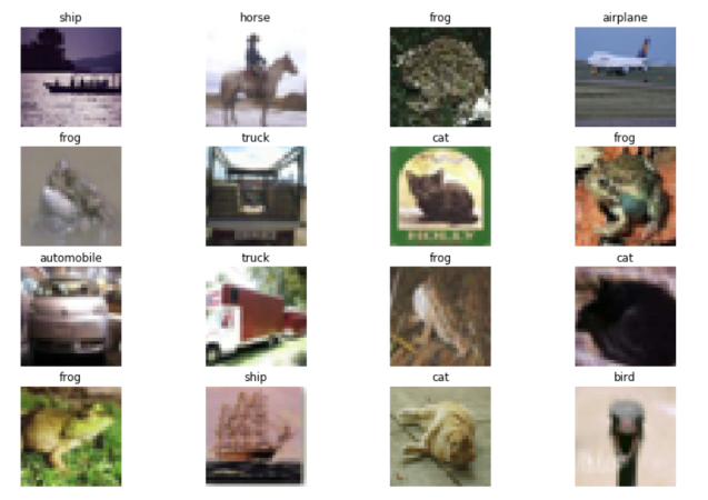
For the purpose of our tutorial we will use the popular cifar-10 data set. It contains 60,000 colorful images in 32×32 pixel format. The images are in low resolution and have been classified into 10 classes: airplanes, cars, ships and trucks, as well as cats, birds, deers, horses, dogs and frogs. Classes are nicely balanced, each of them has 6,000 photos.
The authors of the data set are Alex Krizhevsky, Vinod Nair and Geoffrey Hinton. More about the data set, how it was created and how to use it can be found in this work: Learning Multiple Layers of Features from Tiny Images, Alex Krizhevsky.
Loading the data set is pretty easy because it is available in the keras library:
import numpy as np
import matplotlib.pyplot as plt
import tensorflow
print(tensorflow.__version__)
print(tensorflow.keras.__version__)
>>>2.0.0
>>>2.2.4-tf
from tensorflow.keras.datasets import cifar10
(x_train, y_train), (x_test, y_test) = cifar10.load_data()
The load_data method divides the set into training and test data in a ratio of 50,000 to 10,000.
Let’s check what the first 10 labels look like and what is the shape of the training data:
y_train.shape
>>> (50000, 1)
y_train[0:10]
>>> array([[6], [9], [9], [4], [1], [1], [2], [7], [8], [3]], dtype=uint8)
x_train.shape
>>> (50000, 32, 32, 3)
As you can see the labels are numbers from 0 to 9, where each number represents a given class, e.g. 1 is a car. Training data is an array of 50,000 elements. Each of them contains an image with three channels (RBG) and a resolution of 32×32.
Let’s display 16 randomly selected pictures.
photos_count = 16
photos = np.zeros((photos_count,32,32,3), dtype=int)
desc = np.zeros((photos_count,1), dtype=int)
for i in range(photos_count):
indeks = np.random.randint(0, 50000)
photos[i] = x_train[indeks]
desc[i] = y_train[indeks]
photos.shape
>>> (16, 32, 32, 3)
desc.shape
>>> (16, 1)
A simple dictionary can be used to label the pictures.
dict = {
0: 'airplane',
1: 'automobile',
2: 'bird',
3: 'cat',
4: 'deer',
5: 'dog',
6: 'frog',
7: 'horse',
8: 'ship',
9: 'truck',
}
The matplotlib.pyplot library provides us with extensive data presentation capabilities. We will use a small fraction of these possibilities to present randomly selected 16 photos in one picture:
fig = plt.figure()
for n, (picture, label) in enumerate(zip(photos, desc)):
a = fig.add_subplot(4, 4, n + 1)
plt.imshow(picture)
a.set_title(dict[label[0]])
a.axis('off')
fig.set_size_inches(fig.get_size_inches() * photos_count / 7)
plt.show()
Classification using a classic neural network
Before we get to ConvNets, for reference purposes we will build a classifier on a “regular” densely connected neural network – that is, the one in which each neuron of a given layer is connected to each neuron of the next layer.
Densely connected neural networks expect the input to be “flat”. We have to therefore flatten our colorful images to one-dimensional form. This can be done as below, and you can also use the predefined Flatten layer, which will flatten the data itself. I will use it a little later.
x_train = x_train.reshape((-1, 3072))
x_test = x_test.reshape((-1, 3072))
x_train.shape
>>> (50000, 3072)
The number 3072 results from multiplying the dimensions 32 x 32 x 3.
Because each pixel in each channel determines the intensity of the color component for the pixel, the data should be in the range of 0 to 255. Let’s check this:
x_train.max()
>>> 255
x_train.min()
>>> 0
Neural networks work best in the area of the greatest activity of their activation functions. Therefore, it is good practice to normalize the input data. There are many types of normalization – I wrote more about it here. We normalize the data so that the average falls around 0.
x_train = (x_train / 255)- 0.5
x_test = (x_test / 255)- 0.5
If we wanted to normalize the data around 0.5, the code should look like this:
x_train = (x_train / 255)
Now, all we need to do now is to make necessary imports, build a model, compile it, and start the training process. I wrote in more detail about how to build the model in this post:
from tensorflow.keras.models import Sequential
from tensorflow.keras.layers import Dense
from tensorflow.keras.utils import to_categorical
model = Sequential([
Dense(1024, activation='tanh', input_shape=(3072,)),
Dense(512, activation='tanh'),
Dense(256, activation='tanh'),
Dense(128, activation='tanh'),
Dense(64, activation='tanh'),
Dense(10, activation='softmax')
])
model.compile(
optimizer='RMSprop',
loss='categorical_crossentropy',
metrics=['accuracy']
)
model.fit(
x=x_train,
y=to_categorical(y_train),
epochs=15,
shuffle=True
)
On the training set you should get the accuracy at around 53%.
Let’s check how our neural network will handle test data that it has not previously seen. We will use the evaluate method. If you are wondering why the to_categorical function was used in the fit and evaluate methods, I explained that in this post.
eval = model.evaluate(
x_test,
to_categorical(y_test)
)
eval
>>> [1.5109523288726807, 0.4749]
Our simple neural network on the cifar-10 data set obtained the accuracy of 47%. Given that we have very simple neural network, as many as 10 classes and a relatively low quality images, this is a pretty decent result, especially if we compared it to the 10% offered by a random guess. Having the above benchmark, we could go to ConvNets. However, we will begin by explaining what is a convolution.
Convolution is a mathematical operation
Yeah! Pretty revealing 😉 . Most of what happens in neural networks is in fact a mathematical operation, isn’t? I will add, however, that a convolution is quite simple and has only a few parameters that you only need to be able to interpret to do a convolution yourself.
Let’s start with what is and why we need a convolution at all, since even a simple classic neural network can quite well classify a set and probably if we work on its architecture a bit and add regularization (more on which in the next parts of the tutorial), the result could be much better than 47%.
So what is convolution? I will use some examples. If any of you are interested in music, then certainly you something about sound effects. The original sound can be modified by applying a sound effect filter to it. In the case of an image, which is also a signal, applying a filter can give us the same image, but with certain features highlighted or hidden, e.g. we can sharpen or blur the image, we can also identify the edges on the image. If someone is a fan of photography, she probably used the anti-aliasing effect more than once. It is also nothing else than applying the appropriate filter to the original signal. The operation of applying a filter to a signal is called convolution.
As you can see, there are thousands of uses of the convolution and we don’t realize how often we meet data filtering. However, in the context of image classification and ConvNets, we are interested in a convolution whose purpose is not to enrich the signal (here image) with special effects, but to transform it so that the neural network is able to better capture the characteristics of the image and, as a result, classify it more effectively.
The idea behind a convolutional neural network is to transform the original image before transferring it to a densely connected neural network.
What do we get thanks to a convolution?
- after processing an image with a filter, certain image features are highlighted, which makes them easier to recognize. This is called feature extraction – the network itself finds the features relevant to the image,
- we usually apply many filters at once and each one can highlight different features. For example, when recognizing faces, one will highlight the eyes, the other ears, the hairline or no hair 😉 ,
- as a result of convolution we become independent of the object’s position in the image. Whether the aircraft is presented centrally or in the upper left corner, for the convolutional network will not matter and will not negatively affect the classification. If you read my post about the classification of the MNIST data set, you probably remember that all the numbers were presented centrally there. However, preparing such a “perfect” data set is difficult and time-consuming, and sometimes simply impossible,
- we reduce noise in the analyzed images by focusing the network’s attention on key features,
- usually one of the stages in the convolutional neural network is the layer performing so-called pooling, i.e. combining the values of several adjucent pixels into one. This significantly reduces the computing power needed to train the network without losing important information.
One important note: it is the training algorithm that selects the appropriate filters. This is not our choice as don’t supervise the training process at this level. Filters are randomized and then the back propagation algorithm decides which filter values give the best classification results. As a consequence, the appearance of the image after the machine-implemented convolution often doesn’t say much to the human eye, but it is somehow relevant to the neural network.
Convolution on a single picture
Knowing what a convolution is, before we even use it in neural networks, let’s try to do a convolution on a single photo and see what effects we can achieve.
We will need imports of several libraries, including those for image processing.
import numpy as np
from PIL import Image
import matplotlib.pyplot as plt
%matplotlib inline
We will also define a helper function that will download the image from the local disk, convert it to grayscale, so that we can operate on one and not three color channels and return the whole as a numpy array.
def convert_image(file):
return np.array(Image.open(file).convert('L'))
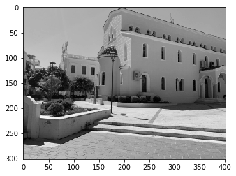
In this example I will use a photo. which I did in the summer of 2019 on Crete. Unfortunately, the gray scale does not reflect how beautiful the sun can be there in September 😎 . The original file (though small in size) for download is available here.
image = convert_image(r'path-to-your-local-directory\house-small.jpg')
image.shape
>>> (302, 403)
plt.imshow(image, cmap='gray')
To implement the convolution we will use keras library:
import tensorflow as tf
print(tf.__version__)
>>> 2.0.0
from tensorflow.keras import Sequential
from tensorflow.keras.layers import Conv2D
We imported a Sequential model and we’ll use the Conv2D layer to implement two-dimensional convolution. The model is very simple – it contains only one layer and a 3×3 kernel (filter). We also need to indicate the size of the input image – we checked it above: 302 x 403.
We perform a convolution using one filter, i.e. the filters parameter should be set to 1.
model = Sequential(
Conv2D(filters=1,
kernel_size=(3,3),
input_shape=(302, 403, 1))
)
The model in the keras library contains a method that can be helpful in understanding how the model looks like.
model.summary()
>>> Model: "sequential"
>>> _________________________________________________________________
>>> Layer (type)                 Output Shape              Param #
>>> =================================================================
>>> conv2d (Conv2D)              (None, 300, 401, 1)       10
>>> =================================================================
>>> Total params: 10
>>> Trainable params: 10
>>> Non-trainable params: 0
It is worth noting the “Output Shape” after convolution, as it is slightly different from the input shape. This is due to the way the convolution operation is carried out. I will not go into details here. More about that in the next part of the tutorial.
Another important issue is reformatting the image so that it is acceptable for the model. The input image is stored in a 302 x 403 array. Meanwhile, the Conv2d layer expects a 4-dimensional tensor. So we need to make the appropriate transformation, for example using the dedicated expend_dims method.
image4Conv = tf.expand_dims(image, 0)
image4Conv = tf.expand_dims(image4Conv, -1)
image4Conv.shape
>>> TensorShape([1, 302, 403, 1])
First, we added the first dimension, whose task is to store the index of the item in the data batch. When we train on large amounts of data, it definitely matters. We have one element / one photo though, so theoretically it doesn’t matter, but keras still expects it to be indexed on the first dimention of the received tensor. The next two dimensions contain the pixel coordinates and the last dimension the pixel value. In our example, we are dealing with shades of gray, i.e. we have one number / one channel. If we were to process an RGB image, the tensor would be of shape [1, 302, 403, 3].
If we were in the training process, the model designed in this way would have to be first compiled by setting the objective function and metrics, and then we would start the training by calling the fit method. However, we just want to pass the image through the Conv2D layer, with filter values randomly selected for now and see what effect we will get. Hence, we will use the predict method, which will do exactly what we want.
result = model.predict(image4Conv)
result.shape
>>> (1, 300, 401, 1)
According to the summary method, we received a 300 x 401 tensor at the output. So the resulting image will be slightly smaller. To display the image we must first get rid of previously added “artificial” dimensions.
result = tf.squeeze(result)
result.shape
>>> TensorShape([300, 401])
plt.imshow(result, cmap='gray')

As you can see the picture was somehow processed by randomly set filter. If you run this or similar code on your environment and work on my image, then you will get a different result, because the randomly set filter will give different final results.
If we want to get a predictable (specific) effect of our convolution, we have to set the filter values ourselves. Keras gives us this option, although in practice it can be rarely used. It is described at the very bottom of this doc page, in the section “Using custom initializers“. It is worth emphasizing once again that the values of the filter are de facto parameters of the model, and the training algorithm changes them in an attempt to obtain the best final results. Thus, the operations we will perform below are only intended to understand the mechanism of convolution. While training the convolutional neural network, we will not interfere with the filter values, although we can initialize these filters in various ways, as described in the link above.
from tensorflow.keras import backend as K
def my_filter(shape, dtype=None):
# We set filter values to detect edges
f = np.array([
[[[-1]], [[-1]], [[-1]]],
[[[-1]], [[ 8]], [[-1]]],
[[[-1]], [[-1]], [[-1]]]
])
return K.variable(f, dtype='float32')
The filter value is set so that it identifies the vertical and horizontal edges, distinguishing them from the other elements of the image. Note that the shape of the filter array is (3,3,1,1) – this may not be visible at first glance – and that the filter elements add up to one. If they didn’t add up to unity, the picture would be darker or lighter. It’s worth experimenting with different filter values. Here is a small note: if you use your image and it is significantly larger than 300 x 400 pixels, then you need to use a slightly larger filter so that the effects of convolution on a larger image are visible to the naked eye.
Now we have to build a model based on the so initiated filter, perform a convolution and display the original and processed images.
model_edge = Sequential(
Conv2D(filters=1,
kernel_size=(3,3),
kernel_initializer=my_filter,
input_shape=(302, 403, 1))
)
result_edge = model_edge.predict(image4Conv)
result_edge.shape
>>> (1, 300, 401, 1)
result_edge = tf.squeeze(result_edge)
result_edge.shape
>>> TensorShape([300, 401])
plt.rcParams['figure.figsize'] = [12, 8]
plt.rcParams['figure.dpi'] = 142
fig = plt.figure()
ax1 = fig.add_subplot(2,1,1)
ax1.imshow(image, cmap='gray')
ax1.set_title('ORIGINAL')
ax2 = fig.add_subplot(2,1,2)
ax2.imshow(result_edge, cmap='gray')
ax2.set_title('AFTER CONVOLUTION')
plt.show()
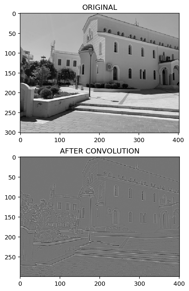
You can see that the convolution has caught most of the edges.
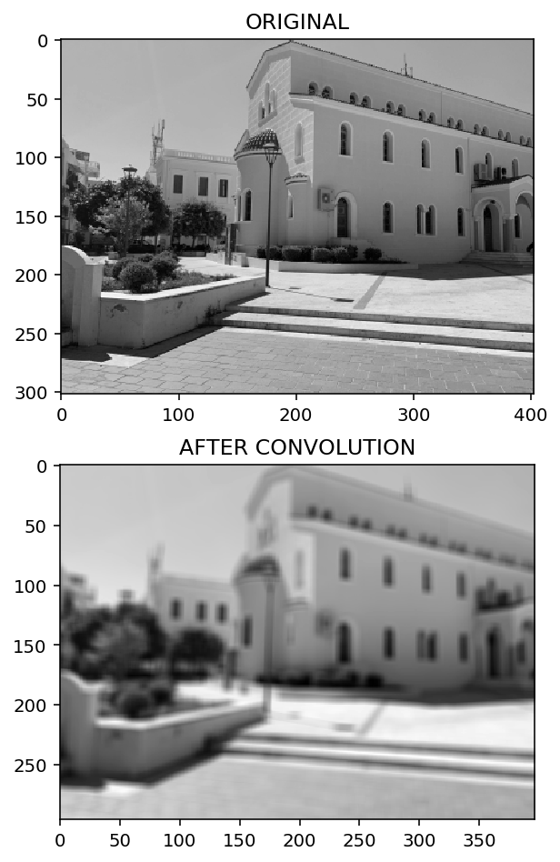
Let’s try another filter that will blur the image. For this purpose, each filter element will have a value of 1 / n, where n is the number of filter elements. For example, for a 3×3 filter, each element should be 1/9. Because I would like the blur to be stronger (more visible), we will use a 7×7 filter with a value of 1/49. In this way, all filter elements still add up to unity.
def my_filter(shape, dtype=None):
f = np.empty(shape=(7,7,1,1))
f.fill(1/49)
return K.variable(f, dtype='float32')
model_blur = Sequential(Conv2D(filters=1, kernel_size=(7,7), kernel_initializer=my_filter, input_shape=(302, 403, 1)))
result_blur = model_blur.predict(image4Conv)
result_blur.shape
>>> (1, 296, 397, 1)
result_blur = tf.squeeze(result_blur)
fig = plt.figure()
ax1 = fig.add_subplot(2,1,1)
ax1.imshow(image, cmap='gray')
ax1.set_title('ORIGINAL')
ax2 = fig.add_subplot(2,1,2)
ax2.imshow(result_blur, cmap='gray')
ax2.set_title('AFTER CONVOLUTION')
plt.show()
Ready to read the next part of this tutorial?
If you liked the tutorial above, please share it or recommend it to your friends.
No Comments