Convolutional neural network 3: convnets and overfitting
Convolutional neural network is one of the most effective neural network architecture in the field of image classification. In the first part of the tutorial, we discussed the convolution operation and built a simple densely connected neural network, which we used to classify CIFAR-10 dataset, achieving accuracy of 47%. In the second part of the tutorial, we familiarized ourselves in detail with the architecture and parameters of the convolutional neural network, we built our own network and obtained ~70% accuracy on the test set. As it turned out, however, we encountered the problem of overfitting, which prevented us from getting better results. In this part of the tutorial, we’ll take a closer look at Convnets and overfitting and inspect various techniques of regularization, i.e. preventing excessive fitting to a training set. We will end the post with a list of practical tips that can be useful when building a convolutional neural network.
From the third part of the tutorial you will learn:
- What is overfitting?
- How to deal with the problem of overfitting?
- What is internal covariate shift?
- How to apply batch normalization?
- What is dropout?
- And some practical tips for building convolutional neural networks.
What is overfitting?
Let’s look again at the results we got in the second part of the tutorial. Figure 1 shows the classification results on the training set, which eventually reached up to ~95% (the blue line). Below there is the classification result for the validation set (the orange line). As you can see, the results for both sets began to diverge already around the 15th epoch, and the final difference for the 80th epoch was as high as ~25%.
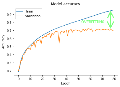
Figure 1 – learning outcomes for training and validation sets
We call this situation overfitting. The network has learned to classify a training set so well that it has lost the ability to effectively generalize, i.e. the ability to correctly classify data that it has not previously seen.
To better understand overfitting, imagine a real life example. A professional basketball player must have the highest quality shoes. He works with a footwear company, and this company prepares shoes that are perfectly suited to the shape and construction of his feet. This requires not only matching the shape of his feet to the shoes, but primarily it requires special insole. Now the basketball player feels great in new shoes and his game is even better. Does this mean that such shoes will be equally good for another basketball player or for amateur players? Probably not in the vast majority of cases. These shoes have been fitted so well to the feet of this particular basketball player that they will not perform well on another feet. This is overfitting, and companies that produce footwear try to design them in such a way that the shapes of the shoes and insoles fit the greatest possible number of feet, while ensuring the greatest comfort of play.
Yet another example – this time graphic. Let’s assume that we want to build a classifier that will correctly classify the data into “circular” and “triangular”.
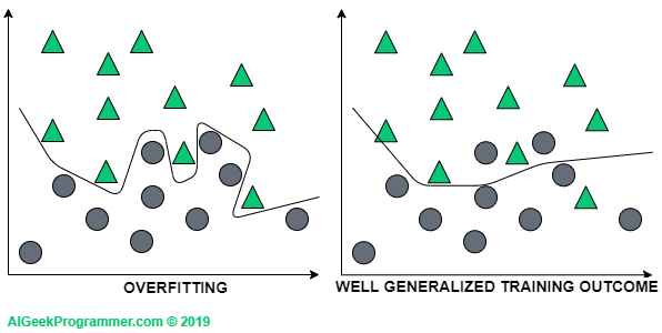
Figure 2 – overfitting vs. better generalizing model
If we adjust the classifier too much to the training data, it will not be able to correctly classify the new data, because it is unlikely that these new data will fit perfectly into the distribution of training data. Therefore, it is better for the model to be less complex. Although it will achieve slightly worse results on the training set, it will probably generalize the problem better, so it will also classify new data more correctly.
How to solve the problem of overfitting?
OK, so how do you counteract overfitting? There are at least several effective methods for this. Below I will describe the most important ones and we will try to use some of them in our classifier.
We collect more data – this is often the most effective method to prevent overfitting. If the model sees more data it will be able to better generalize its response. Let’s remember that neural networks, and in general machine learning, loves huge amounts of data and high computing power. Unfortunately, often this method is the most difficult to use in practice or even impossible – as in our case when we have a closed dataset.
If we can’t collect more data, we can sometimes create it ourselves. Although it sounds quite breakneck and we may wonder if artificially generated data will improve the model’s response, in practice this method brings good results. Especially in image processing we have a wide range of possibilities in that area. We can slightly rotate, move, change its colors or make other more or less subtle changes that will give the model tons of new data. From a logical point of view: having an original photo of a horse, we can mirror it or change its color and it will still be a photo of a horse. This technique is called data augmentation and leading libraries offer ready-to-use tools. We will use one of them in the next part of this tutorial.
As I mentioned in the second part of the tutorial, each neural network has many so-called hyperparameters. They have a significant impact on the way the network works. They are part of the model architecture and by controlling them you can get better or worse results. When building each model, it’s worth experimenting to find architecture that gives us better results. Sometimes reducing the complexity of architecture gives surprisingly good results. Too complex architecture will be able to generate overfitting fairly quickly, because it will be easier for such a network to accurately fit to the training set.
Let’s start with this simple move. The network from the second part of the tutorial consists of convolutional and densely connected subnets. The convolutional network is not densely connected and we should rather try to increase its complexity rather than reduce it, because it will be able to capture more features of the image. Therefore, to reduce the complexity of architecture, it is good idea to start with the densely connected part in the first place.
From the model in the following form (the second part of the tutorial):
Dense(units=512, activation="relu"),
Dense(units=64, activation="relu"),
Dense(units=10, activation="softmax")
we will move to a much simpler one:
Dense(units=32, activation="relu"),
Dense(units=16, activation="relu"),
Dense(units=10, activation="softmax")
(...)
>>> Epoch 78/80
>>> loss: 0.5725 - accuracy: 0.7968 - val_loss: 0.7897 - val_accuracy: 0.7367
>>> Epoch 79/80
>>> loss: 0.5667 - accuracy: 0.8014 - val_loss: 0.8373 - val_accuracy: 0.7259
>>> Epoch 80/80
>>> loss: 0.5611 - accuracy: 0.8019 - val_loss: 0.8255 - val_accuracy: 0.7220
eval = model.evaluate(x_test, to_categorical(y_test))
>>> loss: 0.8427 - accuracy: 0.7164
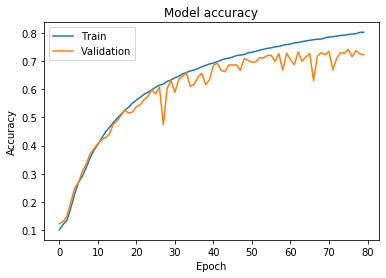
Figure 3 – Training results after reducing the complexity of a densely connected network
As you can see there are some benefits. About 2% higher classification accuracy on the validation set. Faster training, because the network is less computationally demanding. And also reduced, though not eliminated, overfitting – currently at around 10%.
The architecture of our first version of the network, proposed in the second part of the tutorial, assumed the processing of each image by three convolution “modules”, with 64, 32 and 16 filters, respectively. Such a complexity of the convolutional network allowed us to obtain about 80% accuracy on the training set, which translated into ~72% on the test set. For the record, it looked like this:
Convolution2D(filters=64, kernel_size=(3,3), input_shape=(32,32,3), activation='relu', padding='same'),
Convolution2D(filters=64, kernel_size=(3,3), activation='relu', padding='same'),
MaxPool2D((2,2)),
Convolution2D(filters=32, kernel_size=(3,3), activation='relu', padding='same'),
Convolution2D(filters=32, kernel_size=(3,3), activation='relu', padding='same'),
MaxPool2D((2,2)),
Convolution2D(filters=16, kernel_size=(3,3), activation='relu', padding='same'),
Convolution2D(filters=16, kernel_size=(3,3), activation='relu', padding='same'),
In order for us to get better classification results, we should improve in two areas. First, increase the accuracy of classification on the training set, because as you can see the accuracy for the test set is always lower than the accuracy for the training set. Secondly, we should reduce overfitting. A network that learns to generalize well will achieve much better results on data it has not previously seen. In addition, we will be able to train it for more than 80 epochs. Currently, this does not make much sense, because although the accuracy on the training set can still increase, the same parameter on the validation set indicates that this learning is not generalizing, but fitting to the training set.
How to improve the accuracy of classification on the training set? One way is to deepen the convolutional subnet. By adding more layers and increasing the number of filters, we give the network the ability to capture more features and thus greater accuracy in classification. To achieve this, we will add one more convolutional “module” with an increased number of filters:
Convolution2D(filters=128, kernel_size=(5,5), input_shape=(32,32,3), activation='relu', padding='same'),
Convolution2D(filters=128, kernel_size=(5,5), activation='relu', padding='same'),
MaxPool2D((2,2)),
Convolution2D(filters=64, kernel_size=(5,5), activation='relu', padding='same'),
Convolution2D(filters=64, kernel_size=(5,5), activation='relu', padding='same'),
MaxPool2D((2,2)),
Convolution2D(filters=32, kernel_size=(5,5), activation='relu', padding='same'),
Convolution2D(filters=32, kernel_size=(5,5), activation='relu', padding='same'),
MaxPool2D((2,2)),
Convolution2D(filters=16, kernel_size=(3,3), activation='relu', padding='same'),
Convolution2D(filters=16, kernel_size=(3,3), activation='relu', padding='same'),
Attempting to reduce overfitting requires the introduction of two new elements: batch normalization and dropout technique.
Convnets and overfitting: batch normalization
Batch normalization aims to reduce so-called internal covariate shift. To understand the idea behind batch normalization, you must first understand what the internal covariate shift is.
Covariate is a fairly widely used term, mainly in statistics, and means an independent variable, in other words an input variable. On the basis of input variables, output (dependent) variables are determined. By analogy, in machine learning, covariate will mean the input variable / input / X / feature. In our example, covariates are the values of the color components of individual pixels of processed images.
Each dataset has a certain distribution of input data. For example, if in the CIFAR-10 dataset we analyzed the distribution of average brightness of images depicting aircraft, it would probably be different from the brightness of images depicting frogs. If we superimposed these two distributions, they would be shifted from each other. This shift is called covariate shift.
Although the datasets we use for machine learning are usually well-balanced, the division of the set into training, validation and test sets causes that these sets have different distribution of input data. For this reason (among others) we usually have a lower accuracy for the test set as compared to the training set.
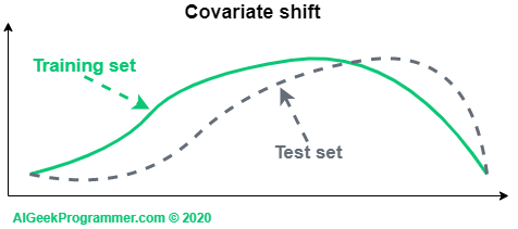
Figure 4 – covariate shift
Covariate shift occurs not only when splitting a set or enriching it with new data, but also as a result of passing input data through subsequent layers of the neural network. The network modifies data naturally by imposing weights assigned to connections between neurons in the network. As a consequence, each subsequent layer must learn data that has a slightly different distribution than the original input. This not only slows down the training process but also makes the network more susceptible to overfitting. The phenomenon of input data distribution shift in the neural network has been described by Ioffe and Szegedy and called internal covariate shift.
Ioffe and Szegedy proposed a method of data normalization performed between layers of the neural network as part of its architecture, thanks to which the phenomenon of internal covariate shift can be minimized. It should be noted here that some researchers dealing with the issue indicate that batch normalization does not so much reduce internal covariate shift, but rather “smoothes” the target function, thus accelerating and improving the training process.
To sum up: batch normalization speeds up learning – allows fewer iterations to get the same results as network without batch normalization. It allows the use of higher learning rates without experiencing vanishing gradient problem and also helps eliminate overfitting. Most machine learning libraries, including Keras, have built-in batch normalization functions.
For those interested: a wiki entry and a scientific article by Sergey Ioffe and Christian Szegedy, who proposed and described the batch normalization method. The article is rather technical, with a large dose of mathematics, but the abstract, introduction and summary are easily understandable.
Convnets and overfitting: dropout
The second very useful technique that effectively fights overfitting is the so-called dropout. It was proposed by Geoffrey E. Hinton, et al. at work Improving neural networks by preventing co-adaptation of feature detectors. It is a relatively simple, but also very effective technique for preventing overfitting. It consists in randomly removing individual neurons from the network (from internal layers, sometimes also input layer) during training. Because complex networks (and these are undoubtedly deep neural networks), especially those with relatively small amounts of training data, tend to accurately match the data, this deregulation method forces them to learn in a more generalized way.
In each training round, each of the neurons is removed or left in the network. The chances of removal are defined by the probability with which the neuron will be removed. In the original work it was 50% for each neuron. Currently, we can independently determine this probability, and for different layers it may be different.
Figure 5 – dropout as a technique to minimize overfitting
The use of dropout in practice leads to a situation in which the network architecture changes dynamically and we get a model in which one dataset was used to teach many networks with different architectures, and then was tested on a test set with averaged weight values.
The use of dropout in Keras comes down to adding another layer called Dropout (rate), whose hyperparameter is the probability with which the neuron will be removed from the network. We add dropouts to the densely connected subnet. Its use in the convolutional subnet is less common and basically misses the idea behind the convolutions.
In the convolution layer, we will use batch normalization, which is obtained in Keras by adding the BatchNormalization () layer. As a result, we will get the following new architecture:
model = Sequential([ Convolution2D(filters=128, kernel_size=(5,5), input_shape=(32,32,3), activation='relu', padding='same'), BatchNormalization(), Convolution2D(filters=128, kernel_size=(5,5), activation='relu', padding='same'), BatchNormalization(), MaxPool2D((2,2)), Convolution2D(filters=64, kernel_size=(5,5), activation='relu', padding='same'), BatchNormalization(), Convolution2D(filters=64, kernel_size=(5,5), activation='relu', padding='same'), BatchNormalization(), MaxPool2D((2,2)), Convolution2D(filters=32, kernel_size=(5,5), activation='relu', padding='same'), BatchNormalization(), Convolution2D(filters=32, kernel_size=(5,5), activation='relu', padding='same'), BatchNormalization(), MaxPool2D((2,2)), Convolution2D(filters=16, kernel_size=(3,3), activation='relu', padding='same'), BatchNormalization(), Convolution2D(filters=16, kernel_size=(3,3), activation='relu', padding='same'), BatchNormalization(), Flatten(), Dense(units=32, activation="relu"), Dropout(0.15), Dense(units=16, activation="relu"), Dropout(0.05), Dense(units=10, activation="softmax")])optim = RMSprop(lr=0.001)
As you can see above, I also proposed to change the optimizer from SGD to RMSprop, which, as shown by my tests, worked slightly better for the above architecture.
Here a small digression: you may be wondering where all these changes come from? Well, they come from two sources: from collected experience and experiments with a given network. I spent at least a dozen hours on the solution that I will finally present in this tutorial, trying different architectures and hyperparameters values. This is how it looks in practice, so if you spend the second day with your model and you have no idea what to do next, then you must know that it is completely normal and in a moment (or after a short break) you will probably go on with your work.
The network has been trained for 80 epochs and as a result we have achieved a classification accuracy of 81%.
Epoch 77/80
42500/42500 - 19s - loss: 0.0493 - accuracy: 0.9888 - val_loss: 1.7957 - val_accuracy: 0.8119
Epoch 78/80
42500/42500 - 19s - loss: 0.0523 - accuracy: 0.9879 - val_loss: 1.2465 - val_accuracy: 0.8016
Epoch 79/80
42500/42500 - 19s - loss: 0.0499 - accuracy: 0.9880 - val_loss: 1.7057 - val_accuracy: 0.8137
Epoch 80/80
42500/42500 - 18s - loss: 0.0490 - accuracy: 0.9880 - val_loss: 1.5880 - val_accuracy: 0.8175
eval = model.evaluate(x_test, to_categorical(y_test))
>>> 10000/10000 [==============================] - 2s 167us/sample - loss: 1.5605 - accuracy: 0.8112
A look at the chart for the training and validation sets gives mixed feelings. On the one hand, we were able to increase the classification accuracy for all three sets, including the most important, i.e. test set, by nearly 10% (from 71% to 81%). On the other hand, strong overfitting has appeared again, which means that the network is again “learning the training set” more than generalizing the classification.
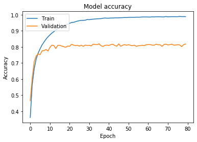
Figure 6 – the result of the classification (changed architecture)
If I wanted to get a better result than 81%, I would choose one of three ways. First, I could experiment with different architectures. I could refer to one of reference architectures that obtained very good results on the CIFAR-10 or similar dataset. Secondly, I could examine the response of the network to other hyperparameter settings – tedious and time-consuming work, but sometimes a few simple changes give good results. The third way is the further fight against overfitting, but with a slightly different method, which I have already mentioned above – data augmentation. We’ll take look at it in the next part of the tutorial.
Convnets – some practical tips
At very the end of this part of the tutorial, I put some practical, loosely coupled tips that you can take into account when building your Convnet.
- If you can, use the proven network architecture and, if possible, adapt it to your needs.
- Start with overfitting and introduce regularization.
- Place the dropout in a densely connected layer and enter batch normalization into the convolutional subnet. However, do not stick to this rule stiffly. Sometimes, non-standard move can give unexpected results.
- Kernel size should be rather much smaller than the size of the image.
- Experiment with different hyperparameter settings, then experiment even more.
- Use the GPU. If you don’t have a computer with a suitable graphics card, use Google Colaboratory.
- Collect as much training data as possible. There is no such thing as “too much data.”
- If you cannot collect more data, use the data generator when possible – more on this in the fourth part of the tutorial.
- A very deep and extensive network will have a strong tendency to overfitting. Use as shallow network as possible. In particular, do not overdo with the number of neurons and layers in a densely connected subnet.
- Ensure that training and test sets are well balanced and have a similar distribution. Otherwise, you will always get much worse results on the test set than on the training set.
- Once you feel good in the Convnet world, start reading more advanced scientific studies. They will allow you to better understand how convolutional networks work, and they will introduce new techniques and architectures to your toolbox.
Good luck! 🙂
I hope you found the above post interesting. If so, share it with your friends.
I invite you to the fourth part of the tutorial.
No Comments